Parallel Processing

Pipelines are executed on clusters of machines. They achieve high throughput by splitting up the work that needs to be done, and then running the work in parallel on the multiple executors spread out across the cluster. In general, the greater the number of splits (also called partitions), the faster the pipeline can be run. The level of parallelism in your pipeline is determined by the sources and shuffle stages in the pipeline.

Autotuning

With each version, CDAP does more and more tuning for you. To get the most benefits from it, you need both the latest CDAP and the latest compute stack. For example, if you are using Dataproc, CDAP 6.4.0 supports Dataproc images version 2.0 and provides adaptive execution tuning. Similarly adaptive execution can be enabled on Hadoop clusters with Spark 3.

For details on how to set the dataproc image version, see this document. Set it to “2.0-debian10” to run Dataproc version 2.0 on Debian 10. 

With adaptive execution tuning, you generally need only to specify the range of partitions to use, not the exact partition number. The exact partition number, even if set in pipeline configuration, is ignored when this feature is enabled.

If you are using an ephemeral Dataproc cluster, CDAP sets proper configuration automatically, but for static Dataproc or Hadoop clusters, the next two configuration parameters can be set:

• spark.default.parallelism - set it to the total number of vCores available in the cluster. This ensures your cluster is not underloaded and defines the lower bound for the number of partitions.

• spark.sql.adaptive.coalescePartitions.initialPartitionNum - set it to 32x of the number of vCores available in the cluster. This defines the upper bound for the number of partitions.

• spark.sql.adaptive.enabled - ensure it’s set to true to enable the optimizations. Dataproc sets it automatically, but you need to ensure it’s enabled if you are using generic Hadoop clusters. 

These parameters can be set in the Engine configuration of a specific pipeline or in the cluster properties of a static Dataproc cluster.

You can find more details at https://spark.apache.org/docs/latest/sql-performance-tuning.html

Clusters

Pipelines are executed on Hadoop clusters. Hadoop is a collection of open source technologies that read, process, and store data in a distributed fashion. Understanding a bit about Hadoop clusters will help you understand how pipelines are executed in parallel. Hadoop is associated with many different systems, but the two used by pipelines are the two most basic ones: HDFS (Hadoop Distributed File System) and YARN (Yet Another Resource Negotiator). HDFS is used to store intermediate data and YARN is used to coordinate workloads across the cluster.

Hadoop clusters consist of master and worker nodes. Master nodes are generally responsible for coordinating work, while worker nodes perform the actual work. Clusters will normally have a small number of master nodes (one or three) and a large number of workers. Hadoop YARN is used as the work coordination system. YARN runs a Resource Manager service on the master node(s) and a Node Manager service on each worker node. Resource Managers coordinate amongst all the Node Managers to determine where to create and execute containers on the cluster.

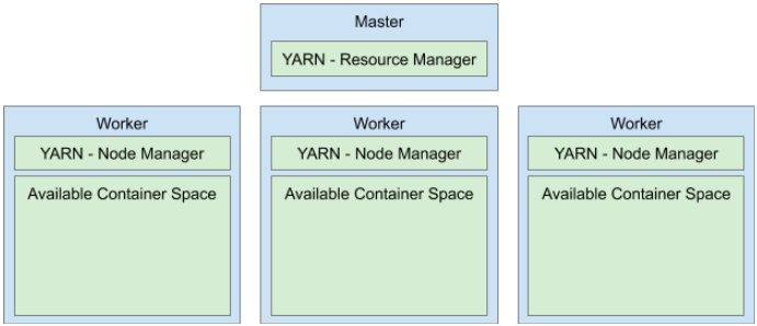
On each worker node, the Node Manager reserves a portion of the available machine memory and CPUs for running YARN containers. For example, on a Dataproc cluster, if your worker nodes are n1-standard-4 VMs (4 CPU, 15 GB memory), each Node Manager will reserve 4 CPUs and 12 GB memory for running YARN containers. The remaining 3 GB of memory is left for the other Hadoop services running on the node.

When a pipeline is run on YARN, it will launch a pipeline workflow driver, a Spark driver, and many Spark executors.

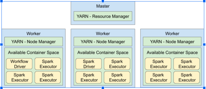
The workflow driver is responsible for launching the one or more Spark programs that make up a pipeline. The workflow driver usually does not do much work. Each Spark program runs a single Spark driver and multiple Spark executors. The driver coordinates work amongst the executors, but usually does not perform any actual work. Most of the actual work is performed by the Spark executors.

Sources

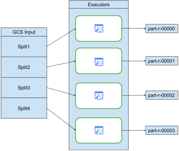
At the start of each pipeline run, every source in your pipeline will calculate what data needs to be read, and how that data can be divided into splits. For example, consider a simple pipeline that reads from GCS, performs some Wrangler transformations, and then writes back to GCS:

When the pipeline starts, the GCS source examines the input files and breaks them up into splits based on the file sizes. For example, a single gigabyte file may be broken up into 100 splits, each 10 megabytes in size. Each executor reads the data for that split, runs the Wrangler transformations, and then writes the output to a "part" file.

If your pipeline is running slowly, one of the first things to check is whether your sources are creating enough splits to take full advantage of parallelism. For example, some types of compression will make plaintext files unsplittable. If you are reading files that have been gzipped, you will notice that your pipeline runs much slower than if you were reading uncompressed files, or files compressed with bzip (which is splittable). Similarly, if you are using the database source and have configured it to use just a single split, it will run much slower than if you configure it to use more splits.

Shuffles

Certain types of plugins will cause data to be shuffled across the cluster. This happens when records being processed by one executor need to be sent to another executor in order to perform the computation. Shuffles are expensive operations because they involve a lot of I/O. Plugins that cause data to be shuffled all show up in the 'Analytics' section of the Pipeline Studio. These include plugins like 'Group By', 'Deduplicate', 'Distinct', and 'Joiner'.

For example, suppose a 'Group By' stage is added to the simple pipeline mentioned earlier:

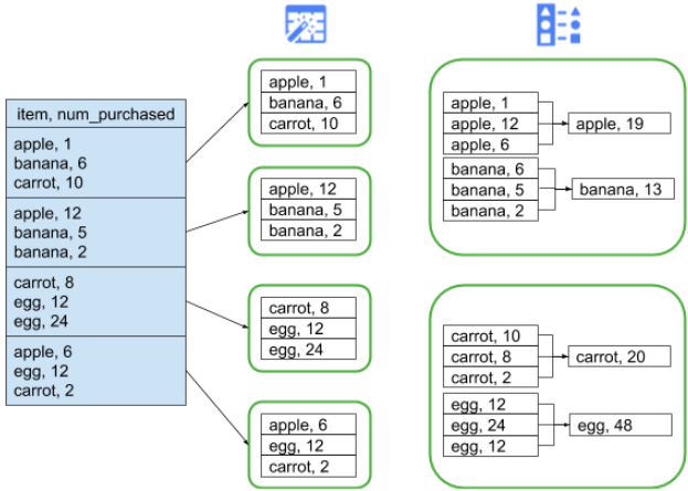
Also suppose the data being read represents purchases made at a grocery store. Each record contains an 'item' field and a 'num_purchased' field. In the 'Group By' stage, we configure the pipeline to group records on the 'item' field and calculate the sum of the 'num_purchased' field:

When the pipeline runs, the input files will be split up as described earlier. After that, each record will be shuffled across the cluster such that every record with the same 'item' will belong to the same executor.

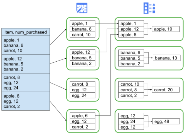
As illustrated above, records for apple purchases were originally spread out across several executors. In order to perform the aggregation, all of those records needed to be sent across the cluster to the same executor.

Shuffle Partitions

Most plugins that require a shuffle will allow you to specify the number of partitions to use when shuffling the data. This controls the number of executors that will be used to process the shuffled data. 

In the example above, if the number of partitions is set to 2, each executor will calculate aggregates for two items instead of one.

Note that it is possible to decrease the parallelism of your pipeline after that stage. For example, consider the logical view of the pipeline:

If the source divides data across 500 partitions but the Group By shuffles using 200 partitions, the maximum level of parallelism after the Group By drops from 500 to 200. Instead of seeing 500 different part files written to GCS, you will see 200.

Choosing Partitions

If the number of partitions is too low, you will not be using the full capacity of your cluster to parallelize as much work as you can. Setting the partitions too high will increase the amount of unnecessary overhead performed. In general, it is better to use too many partitions than too few. Extra overhead is something to worry about if your pipeline takes a few minutes to run and you are trying to shave off a couple minutes. If your pipeline takes hours to run, overhead is generally not something you need to worry about.

A useful, but overly simplistic, way to determine the number of partitions to use is to set it to max(cluster CPUs, input records / 500,000). In other words, take the number of input records and divide by 500,000. If that number is greater than the number of cluster CPUs, use that for the number of partitions. Otherwise, use the number of cluster CPUs. For example, if your cluster has 100 cpus and the shuffle stage is expected to have 100 million input records, use 200 partitions.

A more complete answer is that shuffles perform best when the intermediate shuffle data for each partition can fit completely in an executor's memory so that nothing needs to be spilled to disk. Spark reserves a little less than 30% of an executor's memory for holding shuffle data. The exact number is (total memory - 300mb) * 30%. If we assume each executor is set to use 2gb memory, that means each partition should hold no more than (2gb - 300mb) * 30% ~ 500mb worth of records. If we assume each record compresses down to 1kb in size, then that means (500mb / partition) / (1kb / record) = 500,000 records per partition. This is where the overly simplistic number of 500,000 records per partition. If your executors are using more memory, or your records are smaller, you can adjust this number accordingly.

The following table shows some performance numbers for an evenly distributed join of 500 million records to 1 million records. Each record was roughly 1kb in size before compression. These experiments were performed on a 40 cpu, 120gb cluster, with 2gb executors.

Performance increases until 800 partitions, when shuffle data is no longer spilled to disk. After that, increasing partitions has no benefit on runtime. Note that even a tenfold increase in partitions to 8000 only ends up adding a few minutes of total overhead.

Data Skew

Note that in the example above, purchases for various items were evenly distributed. That is, there were 3 purchases each for apples, bananas, carrots, and eggs. Shuffling on an evenly distributed key is the most performant type of shuffle, but many datasets will not have this property. Continuing the grocery store purchase example from above, we would expect to have many more purchases for eggs than for wedding cards. When there are a few shuffle keys that are much more common than other keys, you are dealing with skewed data. Skewed data can perform significantly worse than unskewed data because a disproportionate amount of work is being performed by a small handful of executors. It causes a small subset of partitions to be much larger than all the others.

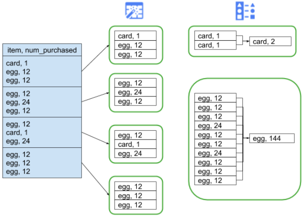
In this example, there are five times as many egg purchases than card purchases, which means the egg aggregate takes roughly five times longer to compute. This does not matter much when dealing with just 10 records instead of two, but will make a great deal of difference when dealing with five billion records instead of one billion. When you have data skew, the number of partitions used in a shuffle will not have a large impact on pipeline performance.

You can recognize data skew by examining the graph for output records over time. If the stage is outputting records at a much higher pace at the start of the pipeline run and then suddenly slows down, this most likely means you have skewed data. 

You can also recognize data skew by examining cluster memory usage over time. If your cluster is at capacity for some time, but suddenly has low memory usage for a period of time, this is also a sign that you are dealing with data skew.

Skewed data most significantly impacts performance when a join is being performed. There are a few techniques that can be used to improve performance for skewed joins. They are discussed later, in the section on joins.